Century version 5
has a new algorithm for erosion, implemented in conjunction with a new deposition
submodel. The Century 4 erosion event
EROD
is still available; the code for handling the event was modified to work
with the new soil physical structure submodel (see the section
Soil Physical Structure Submodel
). The erosion and deposition submodels allow explicit initialization of the
lower layer C, N, P, S pools; erosion and deposition events can cause the thickness
of the simulation layer to vary by changing the depth of the simulation layer-lower
layer boundary. In addition, both layers now utilize the physical properties
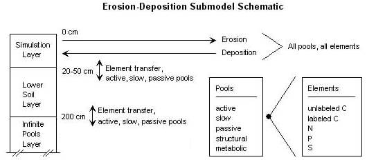
of the soil physical submodel. A schematic of the erosion model is displayed
below; the details of the model are discussed in the following sections.
The simulation layer contains 25 pools (active unlabeled and labeled C, N, P, S; slow unlabeled and labeled C, N, P, S; etc.), while the lower layer contains only the active, slow, and passive pools for each element (15 pools total). Erosion and deposition act upon all 25 pools in the simulation layer, but may cause transfers of the slow, active and passive pools to or from the lower layer. Since the lower layer depth is fixed at 200 cm, pools of infinite capacity are used to provide or accept material in the lower layer as the lower layer thickness expands or contracts; these infinite pools have concentrations equal to the initial values in the lower layer pools.
Deposition events now can be scheduled, using data from a previous simulation
at a site that has undergone erosion. During the simulation with erosion, an
erosion output file is created, which is used for input to the deposition events
in a subsequent simulation. A simulation can have both erosion and deposition
events in the same time step; however, the input for the deposition events
must come (via the erosion file) from a previous simulation. A view of the
element transfers in the erosion-deposition sequence is displayed in the following
diagram:
.
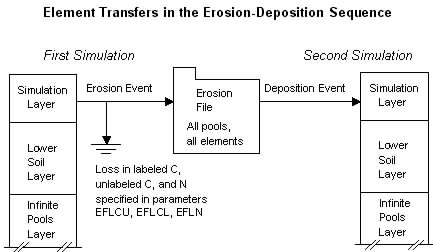
In the first simulation, shown in the figure above, an erosion event results in the amounts eroded from each of the simulation layer pools to be written to an erosion file. Site-specific fractions of C and N lost to dissolution and gaseous diffusion are removed from the eroded pools before the amounts are written to the file. These fractions are specified by the site parameters EFLCU, EFLCL, and EFLN; these are described further in the section, Erosion Output File, below. In the second simulation, a deposition event causes a data record of pool amounts to be read from the erosion file, if the simulation time of the deposition event matches an erosion record's simulation time.
Erosion of, and deposition upon the simulation layer requires a lower layer containing C, N, P, and S pools to act as a source and sink. The upper boundary of this layer is the bottom of the simulation layer. The lower boundary is at the depth of the soil, hence can changed during the simulation along with the soil profile depth and simulation layer thickness. (The simulation and lower layer thicknesses are independent of the physical soil layer thickness, which can be any value equal to or greater than the simulation layer.) The algorithms managing changes to lower soil layer due to erosion and deposition assume a simulation time scale of a few years to hundreds of years, and erosion and deposition rates not exceeding a few mm month-1 of soil thickness.
The lower layer pools are initialized from parameters specified in the site parameters in total g m-2 in the soil below 20 cm depth. These parameters are described in the following table:
| Site parameters specifying the initial pool amounts for the lower layer. | |
| LHICU(1..3) | Unlabeled C for active, slow, and passive pools. |
| LHICL(1..3) | Labeled C for active, slow, and passive pools. |
| LHIN(1..3) | N for active, slow, and passive pools. |
| LHIP(1..3) | P for active, slow, and passive pools. |
| LHIS(1..3) | S for active, slow, and passive pools. |
The Century 4 fixed parameters LHZF(1..3), which are the fractions of the simulation pools with which to initialize the lower layer pools, are used only if a site parameter value for a lower layer pool is less than or equal to zero.
The fixed parameter set contains the parameter EDEPTH, whose value, 20 cm, is both the default and minimum depth for the bottom of the simulation layer. The simulation depth can increase upon deposition to 30 cm. Upon erosion, the simulation depth can decrease to the minimum value (20 cm). As the simulation depth decreases, material is added to the lower layer poolsfrom the infinite pools. The bulk density of the added material, taken from the bulk density of the bottom layer in the physical soil class, is used to calculate the amount of each pool added corresponding to the decrease in the simulation depth, as follows:
| pool amount (g m -2 ) = thickness added (cm) * bulk density of horizon NLAYER (g cm -3 ) * 10000 cm 2 m -2 | (1) |
With the simulation depth at minimum (20 cm), additional erosion transfers material upward, from the lower layer to the simulation layer. The bulk density of the transferred material, taken from the bulk density in the physical soil class over the corresponding depth range, is used to calculate the amount of each pool transferred to the simulation layer. In order to maintain the depth of the lower layer, additional material is added the infinite pools assumed to be below the lower layer and to have the pool densities identical to the initial values for the lower layer.
Upon deposition, the simulation layer depth can increase to 30 cm. As the simulation layer depth increases, material is removed from the bottom of the lower layer and lost. The bulk density of the removed material, taken from the bulk density of the bottom layer in the soil physical class, is used to calculate the amount of each pool removed corresponding to the increase in the simulation depth. With the simulation depth at maximum (30 cm), additional deposition transfers material downward from the simulation layer to the lower layer. When the transfer occurs, homogenization of the lower layer occurs immediately. The thickness of the lower layer can vary. The bulk density of the transferred material, taken from the bulk density in the soil physical class over the corresponding depth range, is used to calculate the amount of each pool transferred to the lower layer, as follows:
| pool amount (g m -2 ) = thickness transferred (cm) * bulk density (g cm -3 ) * 10000 cm 2 m -2 | (2) |
An erosion event, just as in Century 4 schedule files, contains an erosion rate in kg m-2 month-1 in the additional information field. This rate is valid only for this event for which it is specified. Adjustments are made as needed to the lower layer simulation pools, as material is transferred upwards into the simulation layer, and as the simulation layer depth decreases.
A second optional value in the additional information field specifies the enrichment factor, which accommodates the change in organic C content with depth in the simulation layer. Generally, organic C will decrease downward in the simulation layer (the top 20 to 30 cm of soil). The enrichment factor is a positive value greater or less than one. A value greater than one indicates relative enrichment in the top of the simulation layer, while a value less than one indicates relative depletion.
The units for the erosion amount can be quite small. For convenience, note the conversion: g cm-2 = 0.1 * kg m-2. If the bulk density of the surface material is 1 g cm-3, then the event value 0.01 represents a thickness of 0.1 mm.
Another consideration in planning erosion events is the total amount of erosion over the simulated time. The soil will not get thicker without deposition. Over several hundred years of simulation time with erosion, a soil can be too thin to continue the simulation, since the minimum thickness of soil is 20 cm.
The deposition event is new to this version of the model; the additional information field currently is not used. Upon a deposition event, the erosion file is searched for an erosion record of the same simulation time. If found, the amounts are added to the simulation layer according to the algorithm described above. Adjustments are made as needed to the lower layer simulation pools, as material is transferred into it, and as the simulation layer depth increases.
Erosion removes C, N, P, and S that are in the volume of soil removed. A certain amount of this eroded material is permanently lost, as specified by the site parameters listed in the following table. The remainder is written to the erosion output file.
The fractions for the gaseous and dissolution losses are taken from the site parameters EFLCU, EFLCL, and EFLN which refer to an "erosion fraction loss" for unlabeled C, labeled C, and N as described in the table. Each parameter name has an array index to the pool and fraction for the element. The sum of the fractions "gaseous + dissolved" must not exceed 1.0 for each element in a pool. A sum of zero results in the total amount of the eroded element in the pool being written to the erosion file. Conversely, a sum equal to 1.0 results in the none of the element for the pool being written to the erosion file.
These output values are represented in a three-dimensional array: element ´ pool ´ fraction where the dimensions are specified as follows:
| element | Element in the pool: unlabeled C, labeled C, or N. |
| pool | Simulation pools: active, slow, passive, structural, and metabolic. |
| fraction | Fraction of eroded material that is either respired or removed in dissolved form. |
The erosion site parameters are optional. If not specified they are given default values (see the site parameters descriptions for details).
| Site parameters specifying the fractions of an element in a pool lost from the eroded material to gaseous and dissolved pools. | |
| EFLCU(5,2) |
Fraction of unlabeled C in the eroded material lost. The left index is the
pool (active, slow, passive, structural, metabolic). The right index is
the destination (respired, dissolved). E.g.: EFLCU(1,1) = fraction of active unlabeled C in the eroded material lost to respiration. EFLCU(1,2) = fraction of active unlabeled C in the eroded material lost to dissolved organic C. |
| EFLCL(5,2) | Fraction of labeled C in the eroded material lost. The left index is the pool (active, slow, passive, structural, metabolic). The right index is the destination (respired, dissolved). |
| EFLN (5,2) | Fraction of N in the eroded material lost. The left index is the pool (active, slow, passive, structural, metabolic). The right index is the destination (respired, dissolved). |
The erosion output variables in Century 4 named sclosa and scloss have been renamed in this version to EROCCUM and EROC, respectively. They contain the cumulative and monthly C lost to erosion from the sum of the active, slow, passive, metabolic, and structural C pools in the simulation layer.
New output variables are DEPCCUM and DEPC, which contain the cumulative and monthly C gained from deposition into the active, slow, passive, metabolic, and structural C pools in the simulation layer.
A new output variable in the water/temperature group, SIMDEPTH, specifies the depth (cm) of the simulation layer (i.e., the layer thickness) at the time of output.
The Century 4 output variable LHZCAC is still available. This variable contains the cumulative C transferred upward from the lower layer pools to simulation layer pools by erosion (g m-2).
An output file containing values for various pools will be created if a file name is specified in the site management. This file contains the amounts of the pools for C, N, P, and S available for deposition. These are net amounts, calculated as the element amount in the pool after losses due to gaseous diffusion and dissolution.
The output file is in netCDF format and hence cannot be created or viewed using a text editor.You can view the erosion output file in tabular format by (1) translating the file into a comma-separated values format (CSV) using the utility ef2csv, then (2) importing the CSV file into your spreadsheet program. See the description of the ef2csv utility for more details.