The South African Weather Bureau (SAWB) uses advanced climate models to make short-term weather forecasts and long-term forecasts of the climate. The long-term forecasts predict the likelihood of having less rain than normal, normal rainfall, or more rainfall than normal. The SAWB makes forecasts three months in advance, and general predictions about rainfall six months in advance. The utility of these forecasts to farmers of the North-West Province are a topic of our research, reported elsewhere. Here we seek to increase the utility of forecasts by combining them with advanced ecosystem modeling to forecast forage availability and appropriate stocking rates.

To add value to climate forecasts we use the Savanna Modeling System, developed by Michael Coughenour over more than 15 years, to model semi-arid and arid ecosystems. Savanna was designed to model East African grasslands, but now has been used around the world to assist in range management. Savanna combines computer-based maps, weather data, and information on how plants and animals reproduce, grow, and die to predict range condition and animal production. Maps of elevation, soil types, vegetation, and water sources are divided into small blocks (here 1 km x 1 km), and the state of each block is assessed over and over, once for each week being modeled. Each block is further divided into layers of vegetation and soil, so that for example the amount of light passing through each vegetation layer can be calculated and the amount of moisture moving through the soil layers can be modeled.

The long-range forecasts the SAWB produces, and long-range forecasts in general, cannot include specific predictions of rainfall. Instead they produce maps that show the likelihood, reported as probabilities, of a wet, normal, or dry year (Figure 1). In Savanna modeling, we can alter the weather data to represent the forecasted changes in rainfall. Then the ecosystem model provides estimates - forecasts - of range condition, forage availability, and livestock production. We can then change management practices, such as stocking rates, and re-run the computer simulation to find optimal rates.

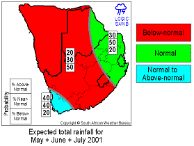Figure 1. A three-month climate forecast for South Africa, forecasting for the North-West Province a 20% chance of a wetter May through July, a 30% chance of normal rainfall, and a 50% chance of the period being dryer than normal (from the SAWB, with permission).

In the North-West Province we are applying the Savanna model to areas representing, in a general way, actual commercial farms in Vryburg 1 and 2, and communal lands in Kudumane, Ganyesa, and Taung. Using vegetation field data collected from around the province by Y. Otsuki, data from interviews of farmers conducted by J. Hudson, information provided to us by South African cooperators, and published data, we have customized the Savanna model to represent 10 farms, 5 commercial and 5 communal. These farms span from being productive to less productive, and understocked to overstocked when compared to recommended levels.

The example that follows represents a 5,900 ha commercial ranch in the southeast portion of Vryburg 1. For this example, the stocking rate of livestock was adjusted to be equal to 8 ha/LSU, as recommended by the Department of Agriculture. Initially there were 726 cattle and 66 sheep, and populations were culled to prevent their numbers from getting too high, and to maintain appropriate sex ratios in the herd. Culling occurred in June, after some animals have died, so cattle were culled if their population exceeded 675, and reset to 626, with the number culled tracked. Of course, modeling can be used to forecast farm conditions in the future, but for this example we use weather patterns from 1970 to 1995 as a guide to the normal variation in rainfall. The region had more than normal rainfall in the mid 1970s, then it was drier than normal through most of the 1980s, and had normal rainfall in the early 1990s. We have varied rainfall during three of those years (from the start of rains in August of one year to the end of rains in July of the following year):
- 1977/1978, near the end of a period of more than normal rainfall amounts;
- 1986/1987, near the end of a period of less than normal rainfall;
- 1991/1992, near the end of a period of normal rainfall;

and for each year, we made the rainfall below normal (225 mm annually), normal (400 mm), and above normal (650 mm) (Figure 2). In this example we focus upon 1977/1978.

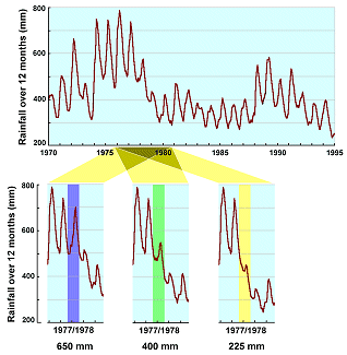Figure 2. The observed rainfall is shown above, with three adjustments made to the rainfall in 1977/1978. In that year total rainfall was adjusted to be 225 mm, 400 mm, and 650 mm, shown below. The peaks in the graphs do not match these values because Savanna calculates rainfall over a long period.

After adapting Savanna to the farm cited, we ran computer simulations over the 25 year period for the drought, normal, and wet rainfall amounts. In general, the simulation responded as would be expected. For example, herbaceous biomass declined dramatically because of the drought (Figure 3).

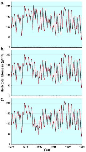Figure 3. Total herbaceous biomass averaged across the farm, when rainfall was above normal (a), normal (b), and below normal (c). Note in (c) how herbaceous biomass declined dramatically during the simulated drought in 1977/1978.

Highly palatable grasses declined relative to low palatable grasses during the drought, and annuals were more likely to become abundant. Cattle populations declined only slightly during the dry mid-1980s when rainfall was abundant in 1977/1978 (Figure 4a), and during the entire 25 year period, 1,507 animals were culled to be sold. With normal rainfall in 1977/1978, cattle declined by about 200 animals (Figure 4b), and 1,328 cattle were culled. When a drought was simulated, cattle numbers declined by half (Figure 4c), and over the entire 25 year period, 1,212 animals were culled.

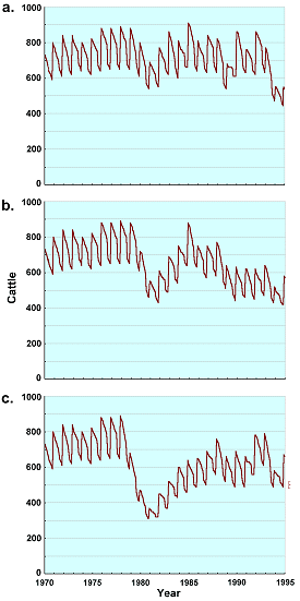Figure 4. The cattle population on the farm, when rainfall in 1977/1978 was above normal (a), normal (b), and below normal (c).

The utility of combining forecasts with modeling farms is demonstrated by adjusting the stocking rate in response to a forecasted drought. SAWB forecasts three to six months into the future, and so a farmer might expect to have a forecast of an upcoming dry season by June. Assuming such a forecast had been received in 1977, we reduced the target population size after culling by 200. Compared to the cattle population when the drought was modeled and the maximum stocking level constant (Figure 4c and the gray line in Figure 5a), removing animals prior to the drought reduced the stress on the range and allowed the livestock to recover more rapidly (the black line in Figure 5a). Further, because the range was in better condition, the population was able to increase during a wet period in the early 1990s (Figure 5a). Over the span of the simulation, an additional 228 cattle were culled to be sold when the forecast was used (Figure 5b), even though the cattle populations were similar at the end of the simulation.

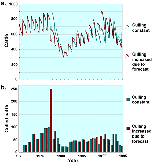Figure 5. Cattle populations with a simulated drought in 1977/1978 are compared (a), when a given stocking rate is maintained (gray line) and when stocking is reduced in response to a long-term forecast (black line). In (b), the number of animals culled (sold) is compared. Some males are culled every year to maintain reasonable sex ratios. Over the entire simulation, 228 more animals were culled when forecasts were used in planning.

Of course, forecasts cannot provide precise estimates of the rainfall that can be expected, and so farmers must judge for themselves the balance between risk and reward. Further, a forecasted drought could reduce livestock prices just as the farmer is considering reducing stocking levels. Forecasts and the economies of farms are addressed elsewhere. Here, we have provided an example of how forecasts linked with an ecosystem model may be useful.